2.1 Basic equations

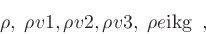
The hydrodynamics equations are expressed as conservation relations plus source terms for

$$\rho, \; \rhov {1}, \rhov {2}, \rhov {3}, \; \rhoeikg \enspace ,$$ (1)

the mass density, the three mass fluxes and the total energy density (per volume), respectively. Each quantity $q$ has its corresponding flux $\mbox{f}(q)$ and possibly source term $\mbox{s}(q)$. For convenience,

$$\rho, \; \V {1}, \V {2}, \V {3}, \; \ei$$ (2)

are chosen as independent quantities. The conserved quantities are purely algebraic combinations of these. The 3D hydrodynamics equations, including source terms due to gravity, are the mass conservation equation

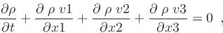$$\papa {\rho}{t} + \papa {\; \rho \; \V {1}}{x1} + \papa {\... ...\; \V {2}}{x2} + \papa {\; \rho \; \V {3}}{x3} = 0 \enspace ,$$ (3)

the momentum equation

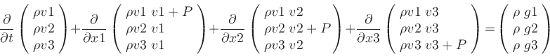$$\papa {}{t} \left( \! \begin{array}{c} \rhov {1} \\ \r... ...\ \rho \; \g {2} \\ \rho \; \g {3} \end{array} \! \right)$$ (4)

and the energy equation including radiative heating term $Q_{\rm rad}$

$$\papa {\rhoeik }{t} + \papa {\; (\rhoeik \! + \! P) \; \V {... ...\g {2} \; \V {2} + \g {3} \; \V {3} ) + Q_{\rm rad} \enspace .$$ (5)

The pressure $P$ is computed from density $\rho$ and internal energy $\ei$ via a (tabulated) equation of state

$$P = P (\rho, \ei ) \enspace .$$ (6)

For local models the gravity field is simply given by

$$\vec{g} = \left( \begin{array}{r} 0 \\ 0 \\ -g \\ \end{array} \right) \enspace .$$ (7)

For global models it is given by

$$\vec{g} = \left( \begin{array}{c} \g {1} \\ \g {2} \\ ... ...\\ \papa {}{x2} \\ \papa {}{x3} \end{array} \right) \Phi$$ (8)

with

$$\Phi = -\frac{G M_\ast}{\left( r_0^4+r^4/\sqrt{1+(r/r_1)^8} \right)^{1/4}} \enspace .$$ (9)

Here, $M_\ast$ is the mass of the star to be modeled; $r_0$ and $r_1$ are free smoothing parameters. In addition, there are equations for the non-local radiation transport. If grey opacity tables are used, the opacities $\kappa$ are a simple function of e.g. temperature $T$ and pressure $P$

$$\kappa = \kappa ( T, P )$$ (10)

and the source function $S$ is given by

$$S= \frac{\sigma}{\pi} T^4 \enspace .$$ (11)

The change in optical depth $\dtau$ along a path with length $\Dx$ is than

$$\dtau = \kappa \rho \Dx \enspace .$$ (12)

The variation of the intensity $\Int$ with optical depth $\tau$ along a ray with orientation $(\theta, \varphi)$ can be described by the simple differential equation

$$\frac{{\rm d} \Int }{{\rm d} \tau} = - \Int + S \enspace .$$ (13)

The radiative energy flux is given by

$$F_{\rm rad} = \int_{0}^{2\pi} \int_{0}^{\pi} \Int \cos \theta \sin \theta \;{\rm d}\theta \;{\rm d}\varphi \enspace .$$ (14)

The energy change can than be computed from the flux divergence with

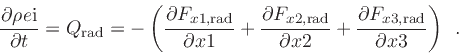$$\frac{\partial \rho e{\rm i}}{\partial t} = Q_{\rm rad} = ... ...ac{\partial F_{x3,\rm rad} }{\partial x3} \right) \enspace .$$ (15)