


Next: 2.3 A collection of
Up: 2. Equations
Previous: 2.1 Basic equations
Contents
Index
2.2 Magnetohydrodynamics (W. Schaffenberger)
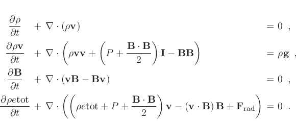
The MHD module solves the equations of ideal MHD, given in compact vector form
 |
(16) |
Here,
 is the magnetic field vector,
where the units are such that the magnetic permeability
is the magnetic field vector,
where the units are such that the magnetic permeability  is equal to one.
 is the identity matrix and
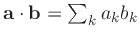 the scalar product
of the two vectors
the scalar product
of the two vectors  and
and  .
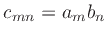
The dyadic tensor product of two vectors
and
is the tensor
.
The dyadic tensor product of two vectors
and
is the tensor
 with elements
 and the
  th component of the divergence of the tensor
  is
is
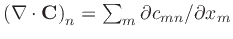 .
The total energy is given by
.
The total energy is given by
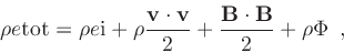 |
(17) |
where  is the internal energy per unit mass.
The additional solenoidality constraint,
is the internal energy per unit mass.
The additional solenoidality constraint,
 |
(18) |
must also be fulfilled.
The aim was to create a stable and easy to use module (Schaffenberger et al., 2005).
The module has the following features:
- Use of the HLL solver with the Janhunen source terms (Janhunen, 2000).
- Extension to 2nd order with linear or parabolic reconstruction and a Hancock predictor
step or Runge-Kutta-TVD timeintegration scheme.
- The following limiters are available: Minmod, vanLeer, Superbee, Piecewise Parabolic (PP).
- Hybridization of 1st and 2nd order flux to ensure positivity of pressure
and density.
- Use of Roe solver.
- Flux interpolated constrained transport step.
- Small violation of strict energy conservation after the constrained transport
step to keep the pressure positive
 -term of Balsara & Spicer (1999).
- Electric conductivity and additional energy diffusion.
- Use of thermal energy equation instead of total energy equation possible
(for HLL solver only).
- Use of both, thermal energy equation and total energy equation possible
(dual energy method, HLL solver only).
- Reduction of Alfvén speed to avoid small time steps (with HLL solver
only and in combination with thermal energy equation or dual energy method only).
- Use of multiple MHD-substeps.
- Boundary conditions for the magnetic field can be specified independently
from the hydro boundary conditions.
- Diffusive boundary layers possible.
- Dimensional splitting or unsplit scheme possible.
The magnetic field is located at the cell boundaries rather than in the cell
centers. Therefore, the format of the magnetic field arrays is slightly
different from that of the other hydrodynamic variables.
Staggered grid representation of the magnetic field in 2 dimensions:
    +---^---+---^---+---^---+---^---+---^---+---^---+
    |       |       |       |       |       |       |
    >   *   >   *   >   *   >   *   >   *   >   *   >
    |       |       |       |       |       |       |
    +---^---+---^---+---^---+---^---+---^---+---^---+
    |       |       |       |       |       |       |
    >   *   >   *   >   *   >   *   >   *   >   *   >
    |       |       |       |       |       |       |
    +---^---+---^---+---^---+---^---+---^---+---^---+
    |       |       |       |       |       |       |
    >   *   >   *   >   *   >   *   >   *   >   *   >
    |       |       |       |       |       |       |
    +---^---+---^---+---^---+---^---+---^---+---^---+
    |       |       |       |       |       |       |
    >   *   >   *   >   *   >   *   >   *   >   *   >
    |       |       |       |       |       |       |
    +---^---+---^---+---^---+---^---+---^---+---^---+
    |       |       |       |       |       |       |
    >   *   >   *   >   *   >   *   >   *   >   *   >
    |       |       |       |       |       |       |
    +---^---+---^---+---^---+---^---+---^---+---^---+

* hydrodynamic variables
> x1 component of the magnetic field
^ x2 component of the magnetic field
The extension to 3 dimensions should be clear. Variables at the left or the
bottom boundary have the same indices as the cell.
For a box with 120 120120 cells, the header for the magnetic field arrays
in the start model may look like
120120 cells, the header for the magnetic field arrays
in the start model may look like
real bb1 d=(1:121,1:120,1:120) f=E13.6 p=4 b=4 &
n='cell boundary magnetic field 1' u=G*sqrt(4pi)
real bb2 d=(1:120,1:121,1:120) f=E13.6 p=4 b=4 &
n='cell boundary magnetic field 2' u=G*sqrt(4pi)
real bb3 d=(1:120,1:120,1:121) f=E13.6 p=4 b=4 &
n='cell boundary magnetic field 3' u=G*sqrt(4pi)
For simplicity, the MHD module uses units such that the 4 pi factors do not
appear in the MHD equations.
Therefore one has to multiply the original magnetic fields in gauss
with the factor  in order to get the correct magnetic field
strength for CO5BOLD!!!
After the computation, one has to multiply the magnetic fields from the
CO5BOLD output with the factor
in order to get the correct magnetic field
strength for CO5BOLD!!!
After the computation, one has to multiply the magnetic fields from the
CO5BOLD output with the factor  in order to get the magnetic
field strength in gauss!!!
The CO5BOLD analysis tool CAT does this automatically when
reading the model data, so that CAT outputs the field strength in gauss.
Positivity of pressure and density:
in order to get the magnetic
field strength in gauss!!!
The CO5BOLD analysis tool CAT does this automatically when
reading the model data, so that CAT outputs the field strength in gauss.
Positivity of pressure and density:
A special problem of MHD simulations is that pressure or density can become
negative in some circumstances. This problem is also present in pure
hydrodynamic simulations but gets worse for MHD.
The original hydrodynamic version of CO5BOLD tries to fix this problem by
reducing the time step. In hydrodynamics, this works in most cases.
In MHD, however, reduction of the time step often does not help and
other methods are necessary to avoid this problem.
Therefore, the MHD module uses a HLL solver instead of a Roe solver,
which is used in the hydrodynamic module (Roe, 1986).
It was shown numerically by Janhunen (2000), that using a HLL
solver together with additional source terms in the induction equation
keeps pressure and density positive under all circumstances.
Because the constrained transport step, which is performed after the
1D sweeps with the MHD solver, changes the magnetic field, a correction of
the internal energy in each cell is necessary to keep the total energy conserved.
Because this correction can lead to negative pressure, it is omitted if
the internal energy would become too small. Therefore, the total energy is not
exactly conserved but this affects only a few cells in the simulation box.
(See also Balsara & Spicer (1999) on this topic.)
The methods described above result in a very robust scheme, which guarantees
positivity of pressure and density under almost all conditions. However,
this does not mean, that these values are accurate! The pressure and
temperature distribution may be very inaccurate in regions with strong
magnetic fields. This may be relevant, if one includes special chromospheric
physics such as dynamic hydrogen ionization and CO formation in the simulation.
A possibility to get more accurate pressure and temperature would
consist in the use of
the entropy equation instead of the energy equation for the computation of the
internal energy in regions with strong magnetic field. This was included in the
original test version of the MHD module. In the present version, we mak use
of the equation for the thermal energy itself depending on the ratio of
thermal to magnetic pressure, i.e., the plasma  . The limiting can
be specified by the model parameter
. The limiting can
be specified by the model parameter beta_inv. This is the dual energy
approach, used in many MHD codes. Its advantage goes at the expense
of violation of strict conservation of the total energy.
Due to the Courant condition, the time step in case of MHD can become
considerably smaller than in the hydrodynamic case. This happens because the
time step is also
limited by the Alfvén speed which is large in regions with strong magnetic
field and low density (small plasma ).
To avoid an extreme time step reduction, the Alfvén speed can be
artificially limited.
This this is done by reducing the Lorentz force in the momentum equation by
a factor f.
This factor is calculated with the following formula:
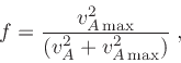 |
(19) |
where  is the original Alfvén speed and
 is the desired maximum
value of the Alfvén speed. Currently, this feature works only with the HLL-solver.
It is advisable to use this feature only in combination with either the thermal
energy equation (
is the desired maximum
value of the Alfvén speed. Currently, this feature works only with the HLL-solver.
It is advisable to use this feature only in combination with either the thermal
energy equation (beta_inv = 0.0) or the dual energy method. In the latter case,
beta_inv should be chosen small enough so that the region where the Lorentz-force
reduction is active is handled by the thermal energy equation. This is obtained
with
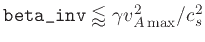 , where
 is the speed of sound and
  the adiabatic exponent.
This module has been extensively tested. It should be able to handle many
MHD flows of astrophysical interest. Bugs and problems can be reported to
the adiabatic exponent.
This module has been extensively tested. It should be able to handle many
MHD flows of astrophysical interest. Bugs and problems can be reported to
werner.schaffenberger@gmx.at.
Next: 2.3 A collection of
Up: 2. Equations
Previous: 2.1 Basic equations
Contents
Index