2.2 Magnetohydrodynamics (W. Schaffenberger)

The current MHD module is a reduced version of the original MHD module. The aim was to create a stable and easy to use module (see [Schaffenberger et al. (2005)]).

The module has the following features:

• Use of the HLL solver with the Janhunen source terms [Janhunen (2000)].
  • Extension to 2nd order with linear reconstruction and a Hancock predictor step.
  • The following limiters are available: Minmod, vanLeer, Superbee.
  • Hybridization of 1st and 2nd order flux to ensure positivity of pressure and density.
• Use of Roe solver.
• Flux interpolated constrained transport step.
• Small violation of strict energy conservation after the constrained transport step to keep the pressure positive $\mathcal{E}$-term of [Balsara (1999)].
• Electric conductivity and additional energy diffusion.
• Use of thermal energy equation instead of total energy equation possible (for HLL solver only).
• Use of both, thermal energy equation and total energy equation possible (dual energy method, HLL solver only).
• Reduction of Alfvén speed to avoid small time steps (with HLL solver only and in combination with thermal energy equation or dual energy method only).
• Use of multiple MHD-substeps.
• Boundary conditions for the magnetic field can be specified independently from the hydro boundary conditions.
• Diffusive boundary layers possible.

The original test version has the additional features:

• HLLC, HLLEM, and Roe solver.
• Janhunen source terms can be deactivated.
• Use of entropy equation instead of energy equation possible.
• Use of both, energy equation and entropy equation possible.
• Field interpolated constrained transport step available.
• Different choices for the energy correction after the constrained transport step: no energy correction, exact energy conservation for each cell or energy correction only if pressure remains positive.

The magnetic field is located at the cell boundaries rather than in the cell centers. Therefore, the format of the magnetic field arrays is slightly different from that of the other hydrodynamic variables.

Staggered grid representation of the magnetic field in 2 dimensions:

    +---^---+---^---+---^---+---^---+---^---+---^---+
    |       |       |       |       |       |       |
    >   *   >   *   >   *   >   *   >   *   >   *   >
    |       |       |       |       |       |       |
    +---^---+---^---+---^---+---^---+---^---+---^---+
    |       |       |       |       |       |       |
    >   *   >   *   >   *   >   *   >   *   >   *   >
    |       |       |       |       |       |       |
    +---^---+---^---+---^---+---^---+---^---+---^---+
    |       |       |       |       |       |       |
    >   *   >   *   >   *   >   *   >   *   >   *   >
    |       |       |       |       |       |       |
    +---^---+---^---+---^---+---^---+---^---+---^---+
    |       |       |       |       |       |       |
    >   *   >   *   >   *   >   *   >   *   >   *   >
    |       |       |       |       |       |       |
    +---^---+---^---+---^---+---^---+---^---+---^---+
    |       |       |       |       |       |       |
    >   *   >   *   >   *   >   *   >   *   >   *   >
    |       |       |       |       |       |       |
    +---^---+---^---+---^---+---^---+---^---+---^---+
    
* hydrodynamic variables
> x1 component of the magnetic field
^ x2 component of the magnetic field

The extension to 3 dimensions should be clear. Variables at the left or the bottom boundary have the same indices as the cell.

For a box with 120$\times$120$\times$120 cells, the header for the magnetic field arrays in the start model may look like

real bb1 d=(1:121,1:120,1:120) f=E13.6 p=4 b=4 &
         n='cell boundary magnetic field 1' u=G*sqrt(4pi)
real bb2 d=(1:120,1:121,1:120) f=E13.6 p=4 b=4 &
         n='cell boundary magnetic field 2' u=G*sqrt(4pi)
real bb3 d=(1:120,1:120,1:121) f=E13.6 p=4 b=4 &
         n='cell boundary magnetic field 3' u=G*sqrt(4pi)

For simplicity, the MHD module uses units such that the 4 pi factors do not appear in the MHD equations.

Therefore one has to multiply the original magnetic fields in gauss with the factor $1/\sqrt{4\pi}$ in order to get the correct magnetic field strength for CO5BOLD!!!

After the computation, one has to multiply the magnetic fields from the CO5BOLD output with the factor $\sqrt{4\pi}$ in order to get the magnetic field strength in gauss!!!

The CO5BOLD analysis tool CAT does this automatically when reading the model data, so that CAT outputs the field strength in gauss.

Positivity of pressure and density:
A special problem of MHD simulations is that pressure or density can become negative in some circumstances. This problem is also present in pure hydrodynamic simulations but gets worse for MHD. The original hydrodynamic version of CO5BOLD tries to fix this problem by reducing the time step. In hydrodynamics, this works in most cases. In MHD, however, reduction of the time step often does not help and other methods are necessary to avoid this problem. Therefore, the MHD module uses a HLL solver instead of a Roe solver, which is used in the hydrodynamic module. It was shown numerically by [Janhunen (2000)], that using a HLL solver together with additional source terms in the induction equation keeps pressure and density positive under all circumstances. Because the constrained transport step, which is performed after the 1D sweeps with the MHD solver, changes the magnetic field, a correction of the internal energy in each cell is necessary to keep the total energy conserved. Because this correction can lead to negative pressure, it is omitted if the internal energy would become too small. Therefore, the total energy is not exactly conserved but this affects only a few cells in the simulation box. (See also [Balsara (1999)] on this topic.)

The methods described above result in a very robust scheme, which guarantees positivity of pressure and density under almost all conditions. However, this does not mean, that these values are accurate! The pressure and temperature distribution may be very inaccurate in regions with strong magnetic fields. This may be relevant, if one includes special chromospheric physics such as dynamic hydrogen ionization and CO formation in the simulation. A possibility to get more accurate pressure and temperature would consist in the use of the entropy equation instead of the energy equation for the computation of the internal energy in regions with strong magnetic field. This was included in the original test version of the MHD module. In the present version, we mak use of the equation for the thermal energy itself depending on the ratio of thermal to magnetic pressure, i.e., the plasma $\beta$. The limiting $\beta$ can be specified by the model parameter beta_inv. This is the dual energy approach, used in many MHD codes. Its advantage goes at the expense of violation of strict conservation of the total energy.

Due to the Courant condition, the time step in case of MHD can become considerably smaller than in the hydrodynamic case. This happens because the time step is also limited by the Alfvén speed which is large in regions with strong magnetic field and low density (small plasma $\beta$).

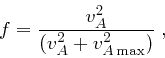
To avoid an extreme time step reduction, the Alfvén speed can be artificially limited. This this is done by reducing the Lorentz force in the momentum equation by a factor f. This factor is calculated with the following formula:

$$f = \frac{v_{A}^2}{(v_{A}^2 + v_{A {\rm max}}^2)}\;,$$ (16)

where $v_{A}$ is the original Alfvén speed and $v_{A {\rm max}}$ is the desired maximum value of the Alfvén speed. Currently, this feature works only with the HLL-solver. It is advisable to use this feature only in combination with either the thermal energy equation (beta_inv = 0.0) or the dual energy method. In the latter case, beta_inv should be chosen small enough so that the region where the Lorentz-force reduction is active is handled by the thermal energy equation. This is obtained with $\verb\vert beta_inv\vert \lessapprox \gamma v_{A {\rm max}}^2/c_s^2$, where $c_s$ is the speed of sound and $\gamma$ the adiabatic exponent.

This module has been extensively tested. It should be able to handle many MHD flows of astrophysical interest. Bugs and problems can be reported to werner.schaffenberger@gmx.at.