 |
 |
|
|||
| STL1001E linearity with temperature dependence 2014 10 30 |
| Telescope setup | The test was conducted in dusk to early evening with the dome closed and curtains to the upper control room down. The dome was rotated to the initial position and the telescope was stopped, pointing towards the dome flat screen (ALT:98 AZ:22, telescope value). Furthermore, the 80cm mask was on, the secondary had it's 42cm ring (used for scatteredlight measurement), and the tertiary had it's 32cm ring (used for scatteredlight measurement). The light source used was the two modified flat screen lamps (Diffuse light lampholder for the flatfield screen), shining from underneath the front end of the telescope towards the flat field screen. The single pixel intensity roughly corresponds to the combined flux from a 15mag star, or the maximum value of a 12.4mag star (seeing 3.3), or about 19 times the background during astronomical night. The ST1001E camera was mounted in the left focus with F/10 setting, and with tubes B and D. The rotation was about 0 position in angle relative to the telescope (Focus value 28) and with derotator tracking off. | Observation | Three data series was taken at TCCD=-10°C, -20°C, and -30°C (in that order, also here after referred to as set 1, 2 ,3). Each sequence consisted of single exposures 5, 10, 20, 30, 40, 50, 60, 70, 80, 90, 100, 110, and 120 seconds long. After (and therefore also between) each exposure a 120s DARK was taken (13 in total), and the sequence ended with 13 BIAS frames. No filter was used. The reason for this sequence is that the CCD retains a lasting imprint of the former exposure, or has a pixel sensitivity change when exposed. This investigation is not intended to investigate this behavior but it is an opportunity to gather some data which might be useful and sequence will give a sort of mean DARK for all exposures. The sequences went between 14:52-15:35UT, 15:54-16:37UT, and 16:50-17:33UT. Most of the in between time is for the CCD cooling to settle. The dome is not fully light tight, thus due to the faint light there is a small risk that out side light might have contributed. The light from the flat field lamps is assumed to be constant. |
Reduction | All Bias frames within each temperature set were averaged into a master BIAS. In the same way, all DARKs were averaged, master BIAS subtracted, and scaled (divided) to 1s into a master DARK. All light frames were then subtracted by the corresponding master BIAS, and subtracted by the correct master DARK, scaled to the exposure time of the light frame. In this investigation there were no need for flats since the interest is in how the ADU counts relates to the exposure time and not measuring the light source. In this procedure there is no detection of secondary sources for ADU contribution e.g. cosmic hits. For this purpose a pixel mask was created for each temperature set where suspicious pixels were marked. The first step was to remove pixels with ADU above 65,000 (i.e. very close to saturation) in the raw frames of either of the BIAS, DARK or light frames. A second sweep is done to detect pixels affected by low level cosmic rays in the following way:
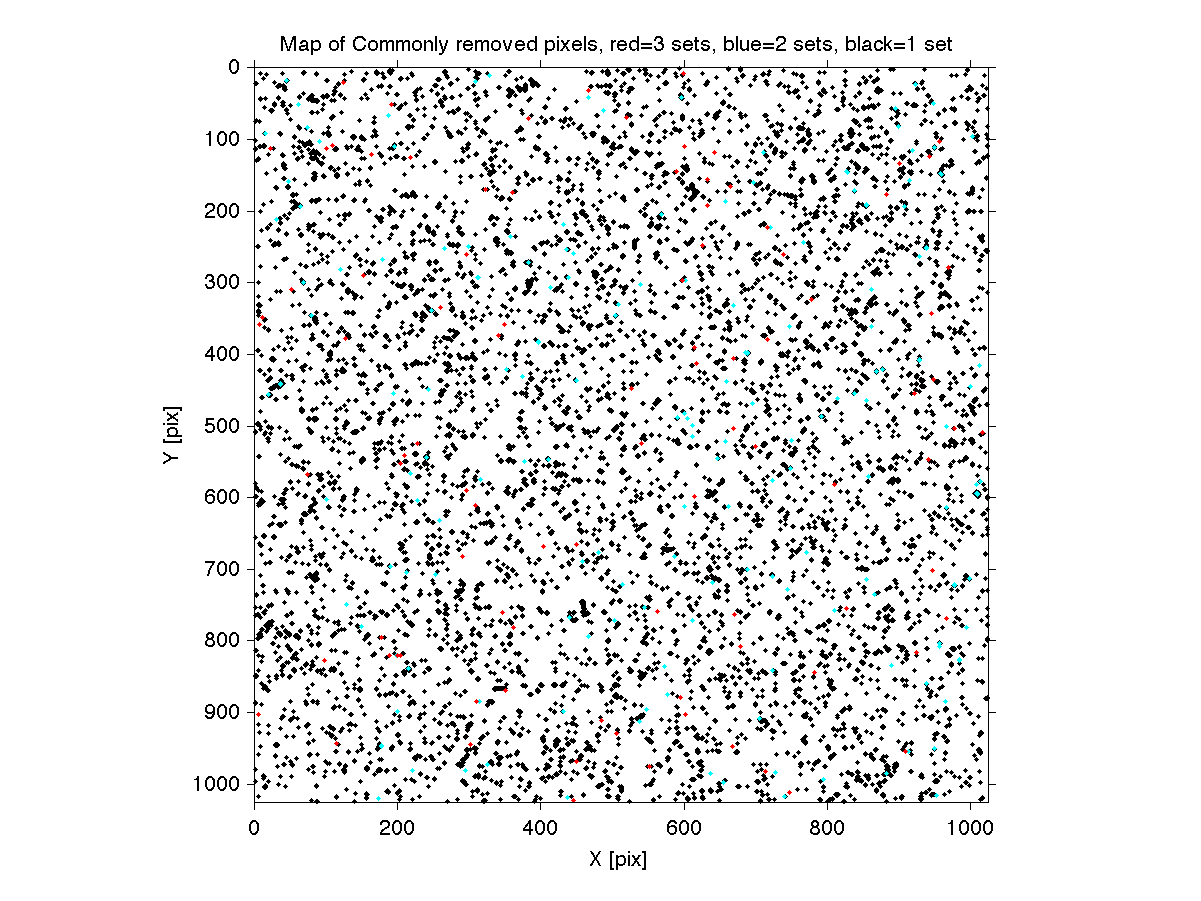
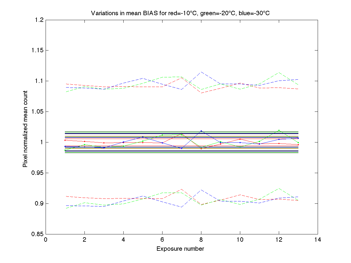
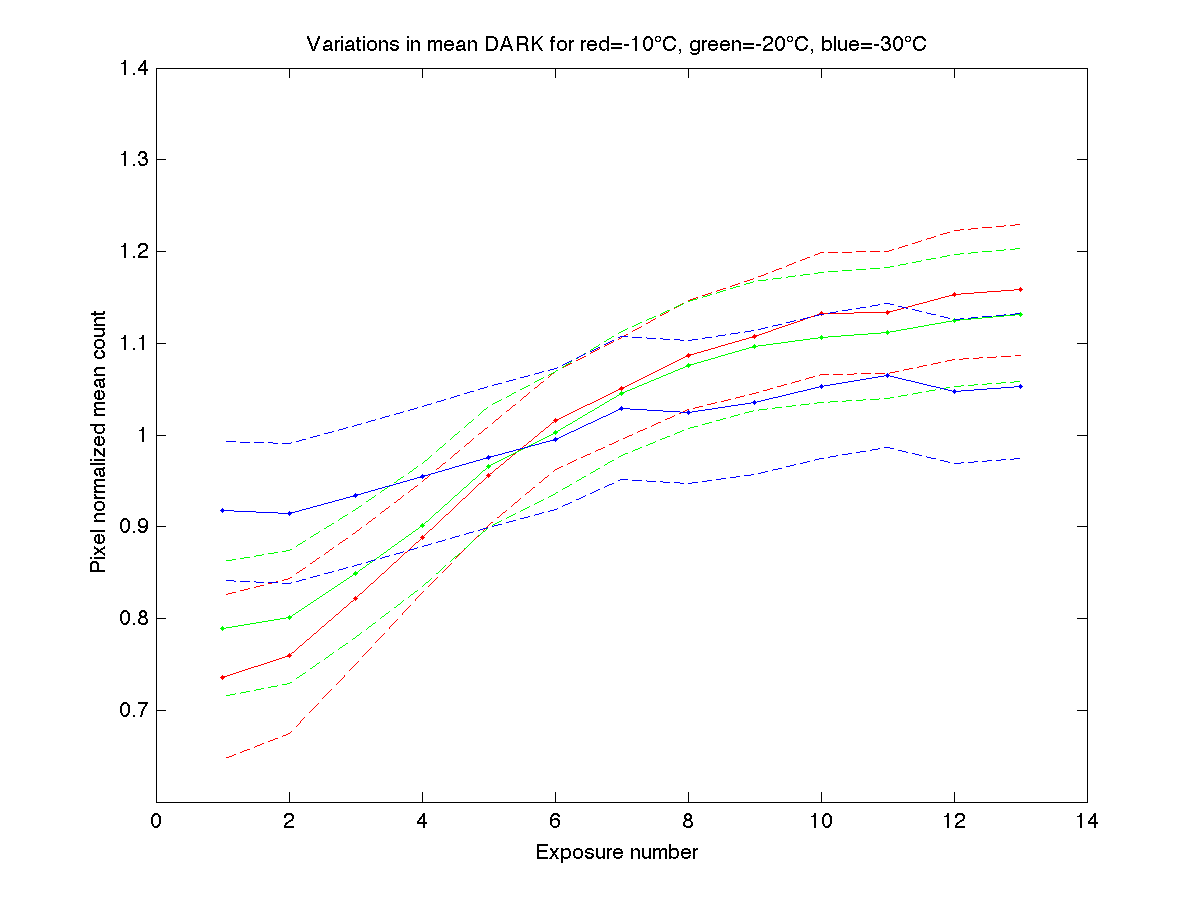
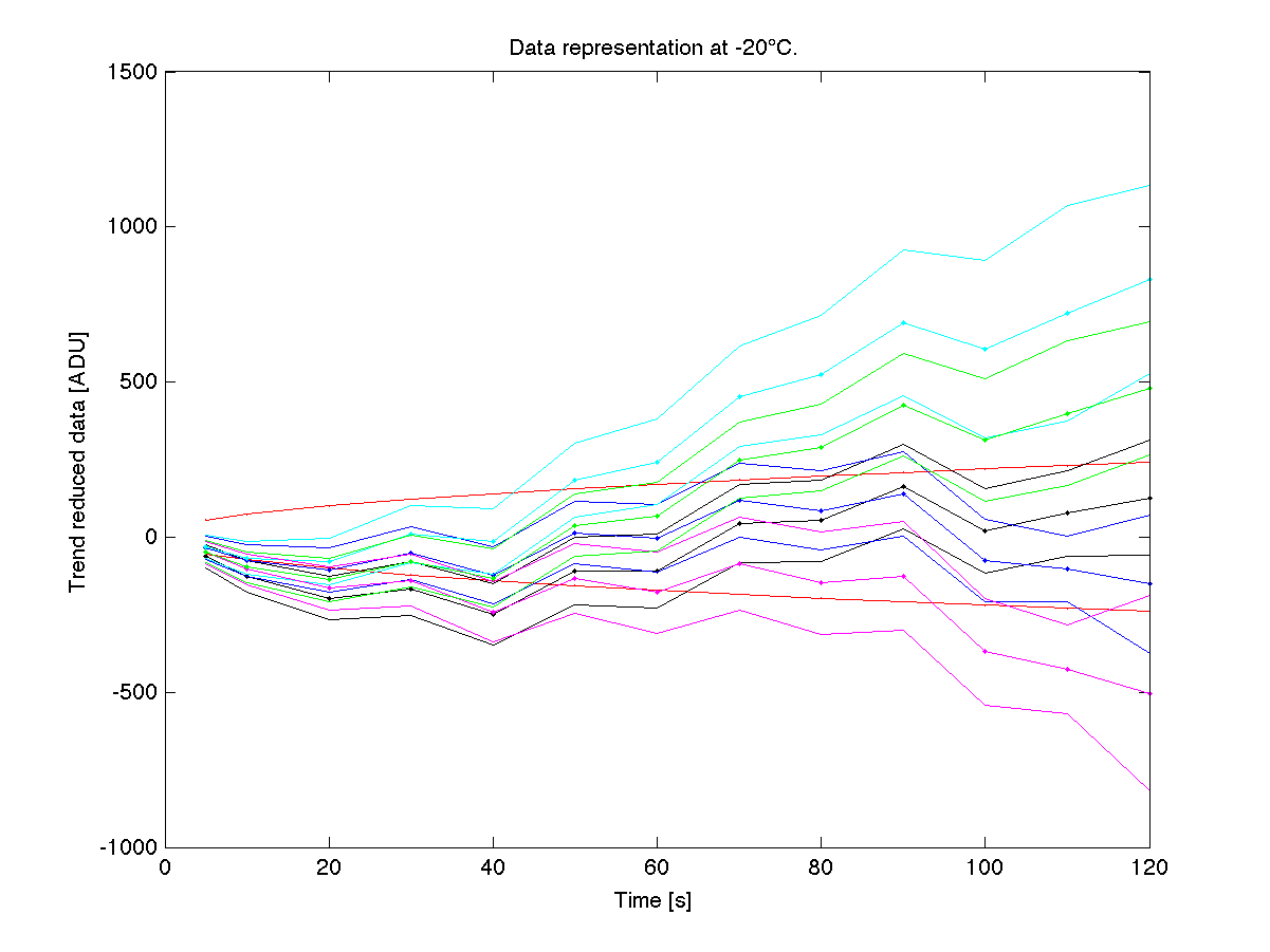
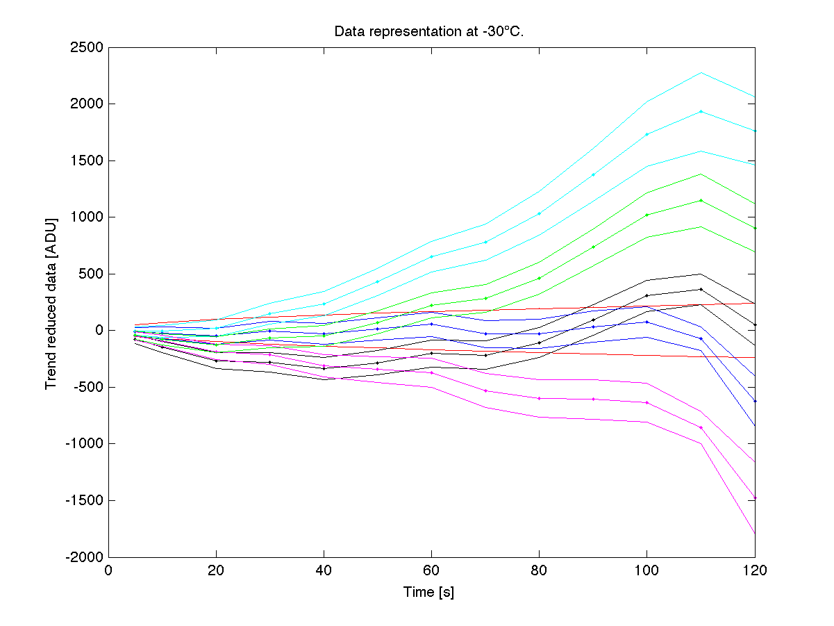
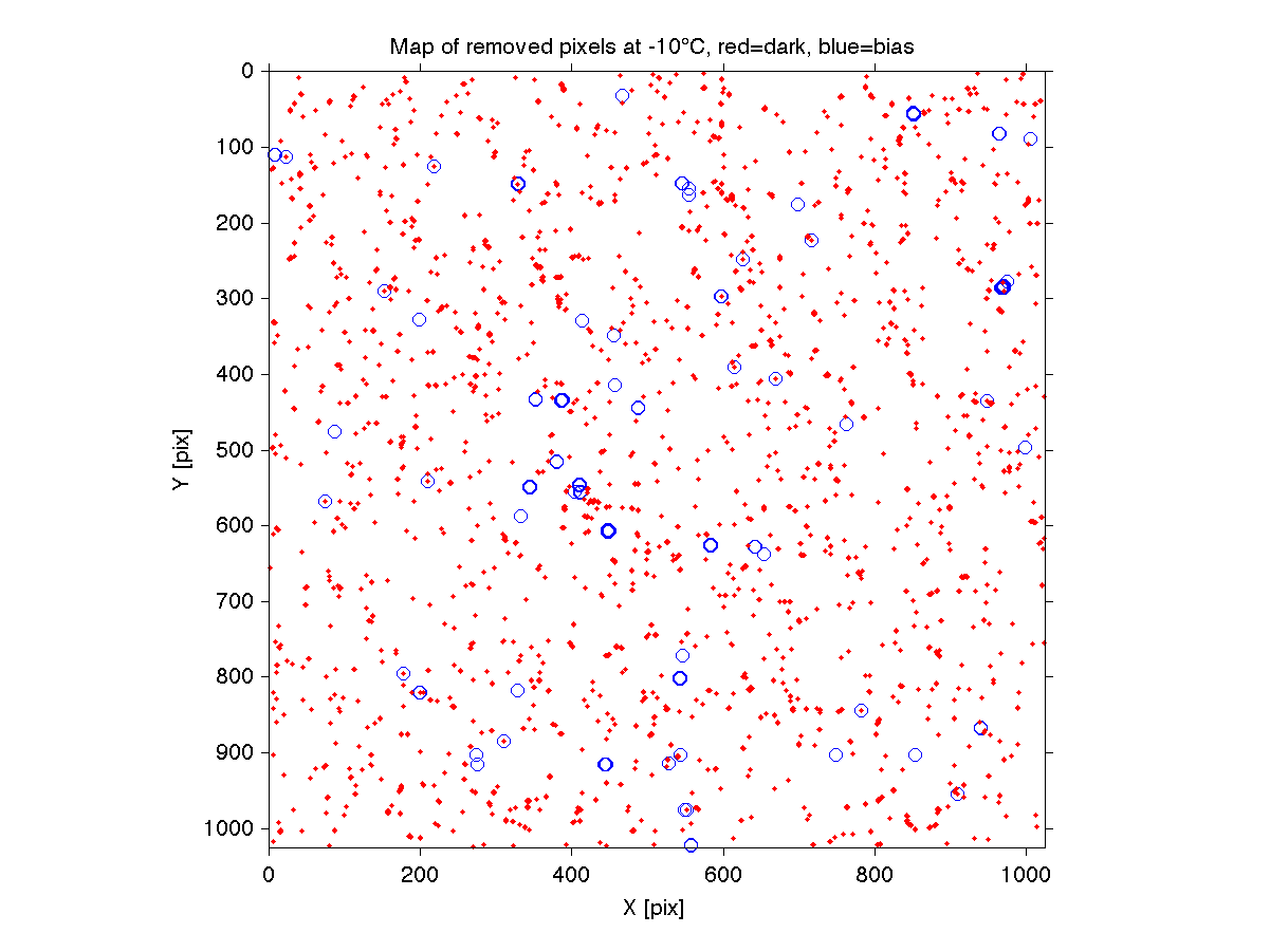
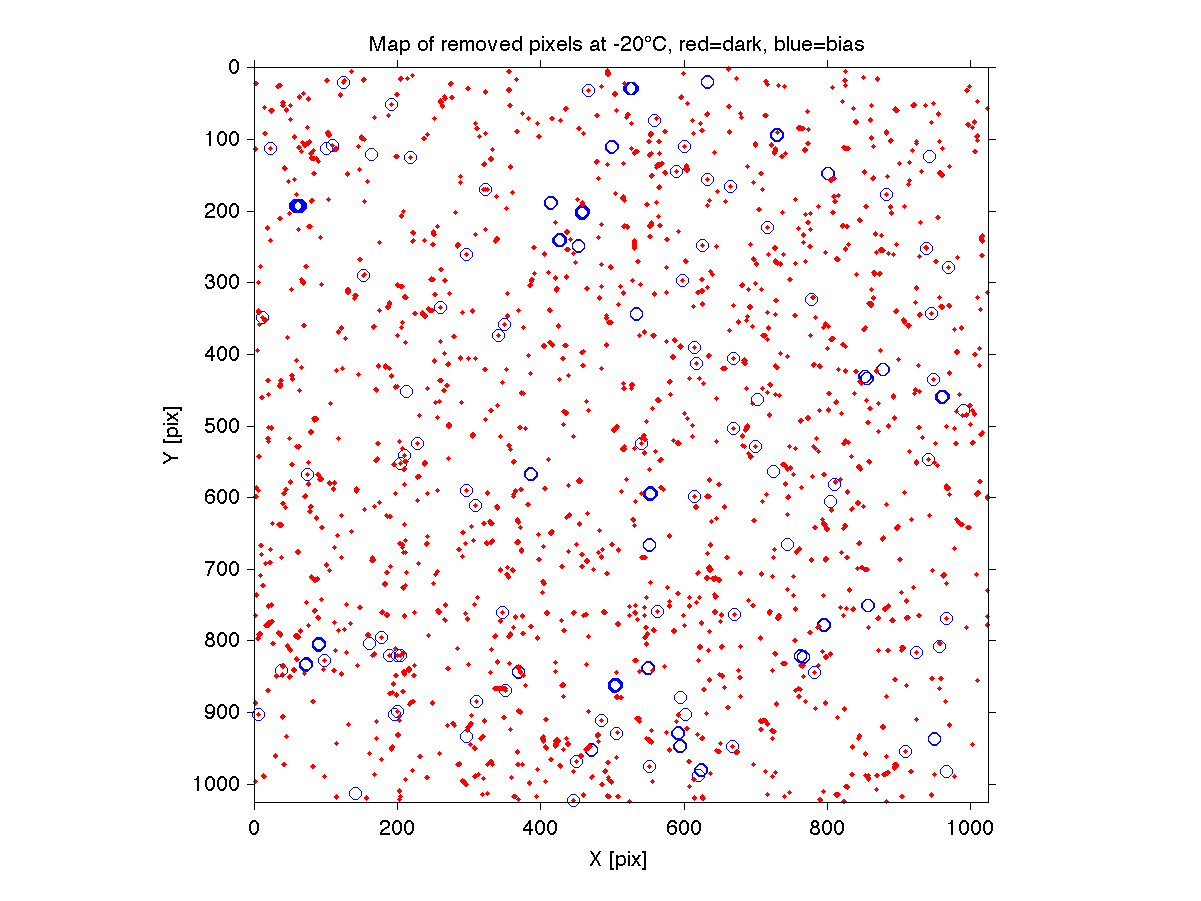
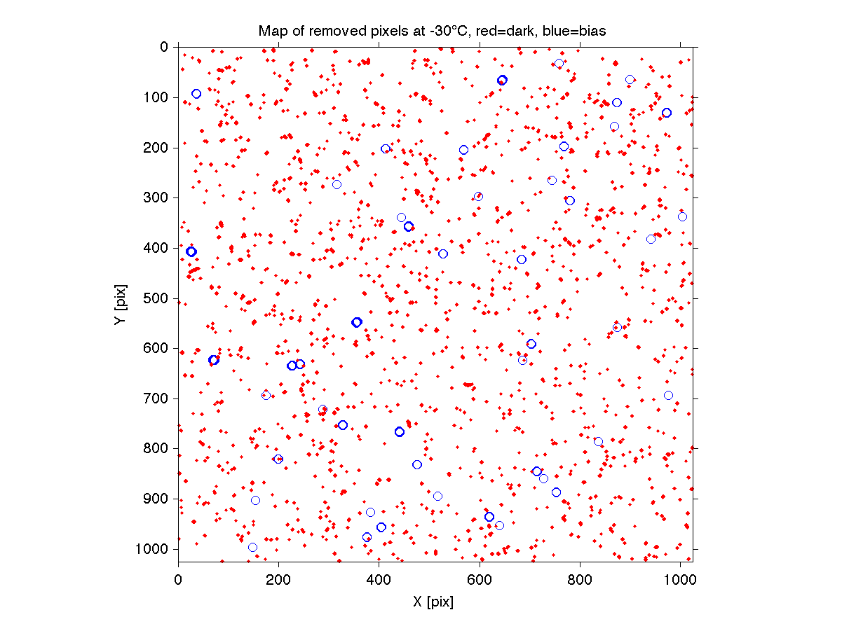
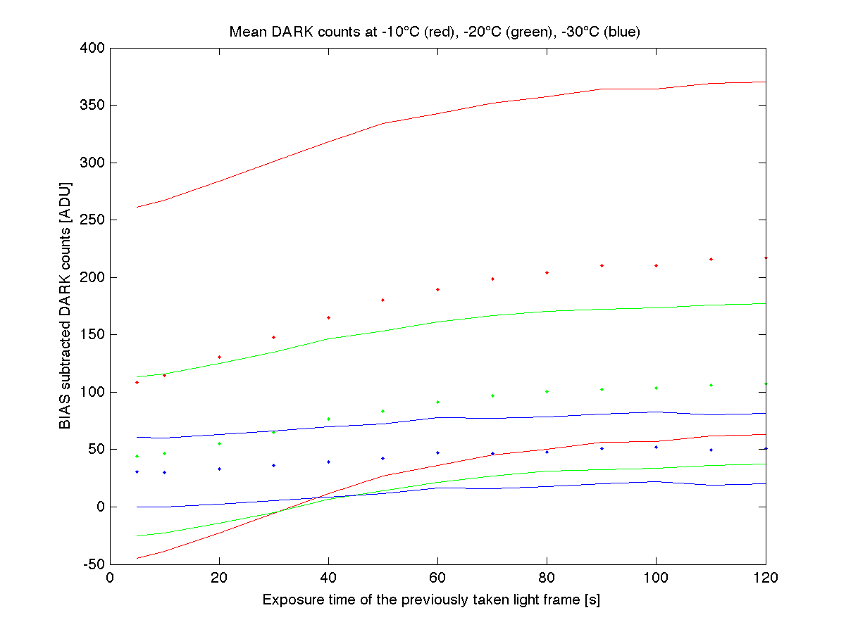
The same method cannot be directly used for the light frames because of the natural variation in counts due to the different exposure times. Instead the reduced light frames are used which first are scaled to the same exposure time (1s), after which the pixel standard deviation can be calculated similar to the BIAS and DARK frames. This will naturally also includes effects from the subtracted master DARK and master BIAS. However, since the affected pixels are already marked, marking them again will have no additional affect. In this case 12246 pixels were masked (Table 1) i.e. the combination of all dots in Fig 1.. This is about 1.2% of all pixels. However, only a small fraction of the masked pixels are present in more than one map, indicating possible physically troublesome pixels (cyan and red dots). In total it represents an exposure of about 2.6h. Most mapped pixels are most likely the result of cosmic hits.After the mapping of troublesome pixels the reference images can be examined. In Fig. 2 the mean BIAS have been plotted after first normalized with respective pixel average. The dashed lines show one sigma deviation for the three data sets (red=-10°C, green=-20°C, blue=-30°C) within each frame. Some of this deviation is caused by the systematic variations in the BIAS frame. One such systematic effect is that DARK electrons continues to be collected during readout. Another effect is that the sensitivity are slightly different from pixel to pixel. The solid lines (colored) show the deviation in the mean of each set at one sigma and (further away from ordinate of 1) the expected limit for one data point. The solid black line is the corresponding uncertainty limits for the total set at one sigma and for three, two, and one data point. The only data set that shows a slight deviation from noise is the -10°C case where there are two points deviating more than expected. However, this is the result of the rest of the data points being closer to the mean line at one than seen in the other two sets. Compared to the other data sets or to the total set, things are close to the expected outcome of random variations. The deviations within each frame, the dashed lines, also follows the mean values. If some pixels would have behaved significantly different in some frames causing a shift in the mean value it would have increased the uncertainty in that frame, and furthermore should already have been removed to the mask, thus the BIAS frames raises no concerns.The same cannot be said about the DARK frames. As can be seen in Fig. 3, the deviation is obvious. Since the DARK frames are taken with the same exposure time the data should be gathered around a horizontal line. This is a clear indication that the reduced data will not be linear. However, due to previous tests with the camera this is expected, and one of the reasons to check the linearity in the first place. In fact there are three effects which are expected to be present and affecting the linearity.
|
Theoretical model |
The next step is to introduce a model to describe the function y=f(t,T) for each pixel, where y stands for the pixel intensity/counts (ADU), t is the time (s), and T is the temperature (°C). Because the possible nonlinearity behavior is studied a simple model y(t)=At2+Bt, yi=Ati2+Bti, (Eq. 1) is chosen, where (yi,ti) are the data points (count [ADU], time [s]) for a specific pixel and the temperature is kept constant. If the relationship is linear then A is zero i.e. A gives the estimation of the nonlinearity. However, the incoming intensity might be different on different pixels so in order to give a general behavior description of the CCD rather than a pixel by pixel behavior the data needs to be assimilated in some way. The parameter can be presented by normalizing it with respect to the slope B A drawback by using this quadratic model is that the nonlinear effect is always present (and has a square dependence), while this might not be the case in reality. To compensate/check this different upper/lower cuts in the counts can be applied before fitting the data to the model and then the parameter trend can be examined. Because of the term A in Eq. 1 the slope B might be over compensated if the relationship is nearly linear. If A is negative it can be compensated by letting B be more positive than if A was zero. In order to cope with this a strict linear relationship can be used. Of course this will have the opposite problem to Eq. 1 because it cannot track nonlinearities, but as described above the trend can be checked by using subsets of the data. The data fit to Eq. 1 in least square sense, assuming no deviation in time t is (Eq. 4)The fitted parameters A and B are collected for each pixel p. The uncertainty of A and B can be estimated by differentiation (Eq. 5)Following the same routine the fit to Eq. 3 is (Eq. 6)
Top left: -10°C case. The data is bending in two ways first positively and then negatively. One or two of the last points might have been affected by a general shift. Neither the linear, nor the quadratic model can fully represent the data. The quadratic model have a general negative quadratic term compensated by a too positive linear term, hence the negative values. The mean linear term is not a good representation of the data either. Top right: -20°C case. The Quadratic model can marginally represent the data. The data starts with a positive bending which levels out at the end. The Quadratic term is generally positive. The linear model is slightly worse in representing the data compared to the quadratic model. Bottom left: -30°C case. The quadratic model is a fairly good fit i.e. the data is by no mean linear. The deviation of the last point might be a general shift of the data, or the third of the expected nonlinear effects. 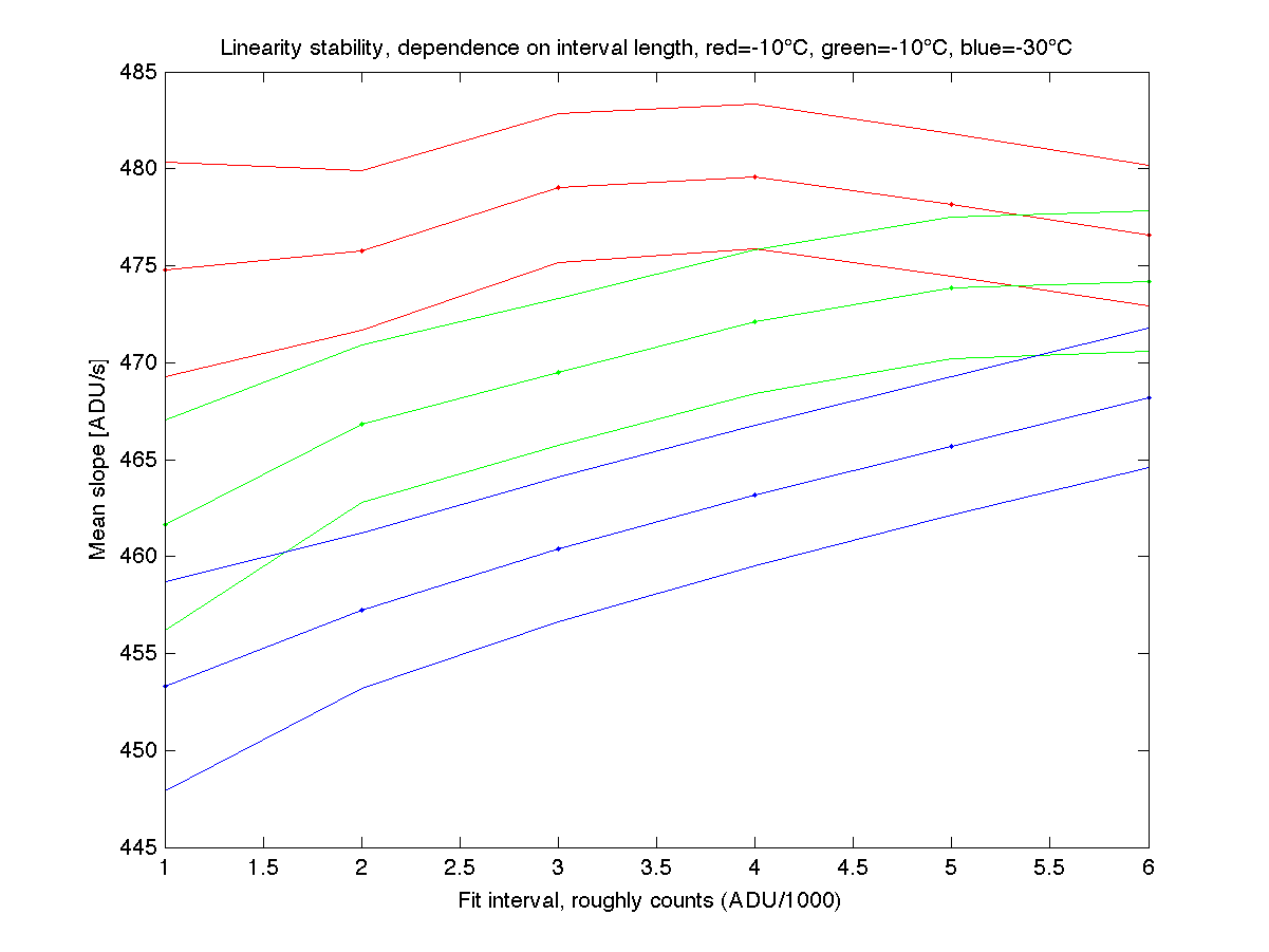 Fig.5 Mean linear slope variations among p pixels depending on number of the data points per pixel used, counted from the shortest exposure time. so that Yp(t)=Dpt represents the number of counts as a function of time for each pixel given the constant light source used in this situation. Although the full data series have a stronger weight it should be to some extent compensated by the "noisier" shorter data series in case their behavior is more linear than the full series. This should work for the red case in Fig. 5 but as can be seen the green and the blue cases have a steady increase in the slope term i.e. the weighted value will favor a higher value than the ordinary mean. Because this behavior actually comes from the nonlinearity along the whole dynamical range of the CCD this probably places the linear proxy away from its true value. On the other hand this value is not known anyway. Furthermore, the different temperature sets do not give any indication of where the value should be placed. The first series is the red one, with a fairy constant mean value. After a bit of further CCD cooling comes the green series where the slope increases with time but again is reduced after further cooling. The gap between red and blue represents a difference in slope of about 4% which directly relates to a difference in counts, although the light source should be constant. Since Eq. 1 is supposed to represent the actual behavior, the difference to the linear approximation in Eq. 7 can represent the nonlinearity of the pixel ΔYp=At2+(B-Dp)t. |
Result |
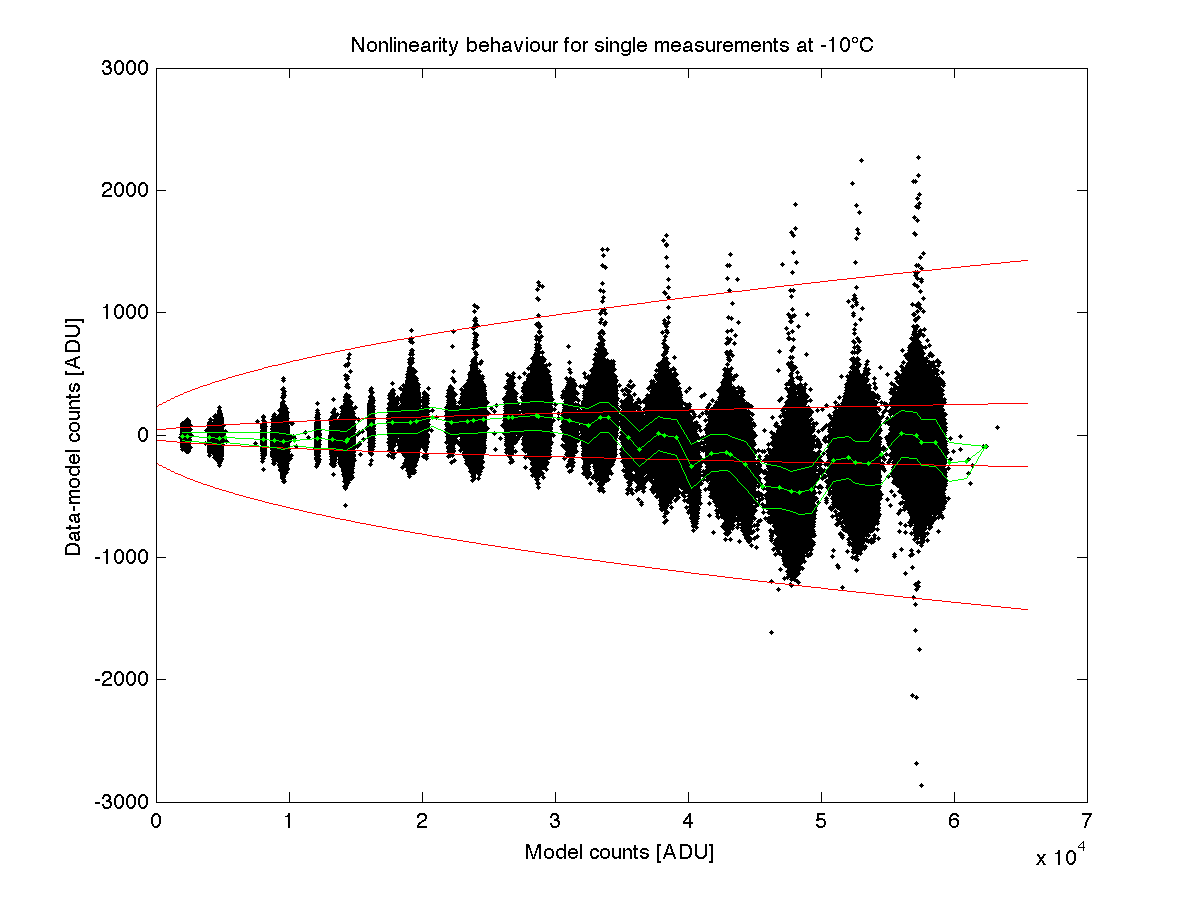
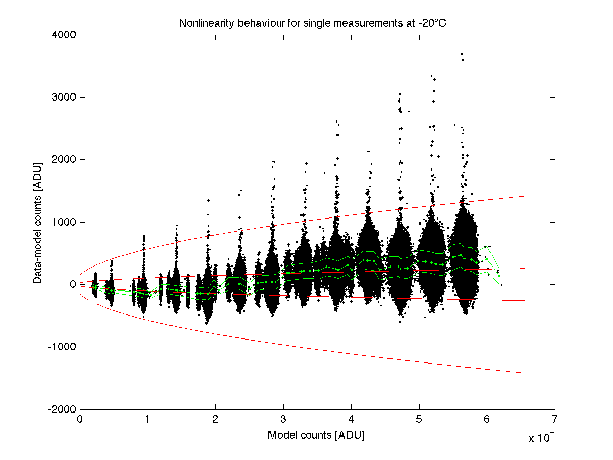
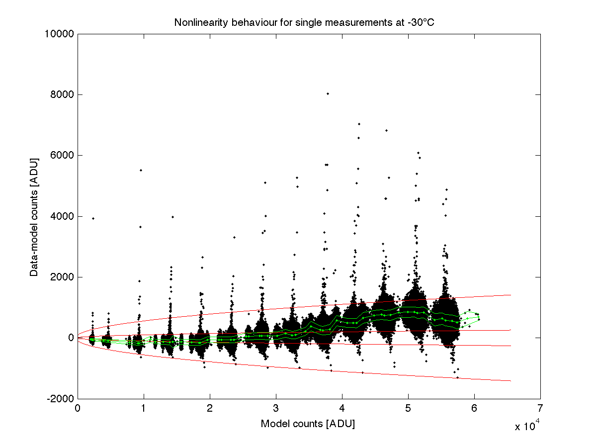
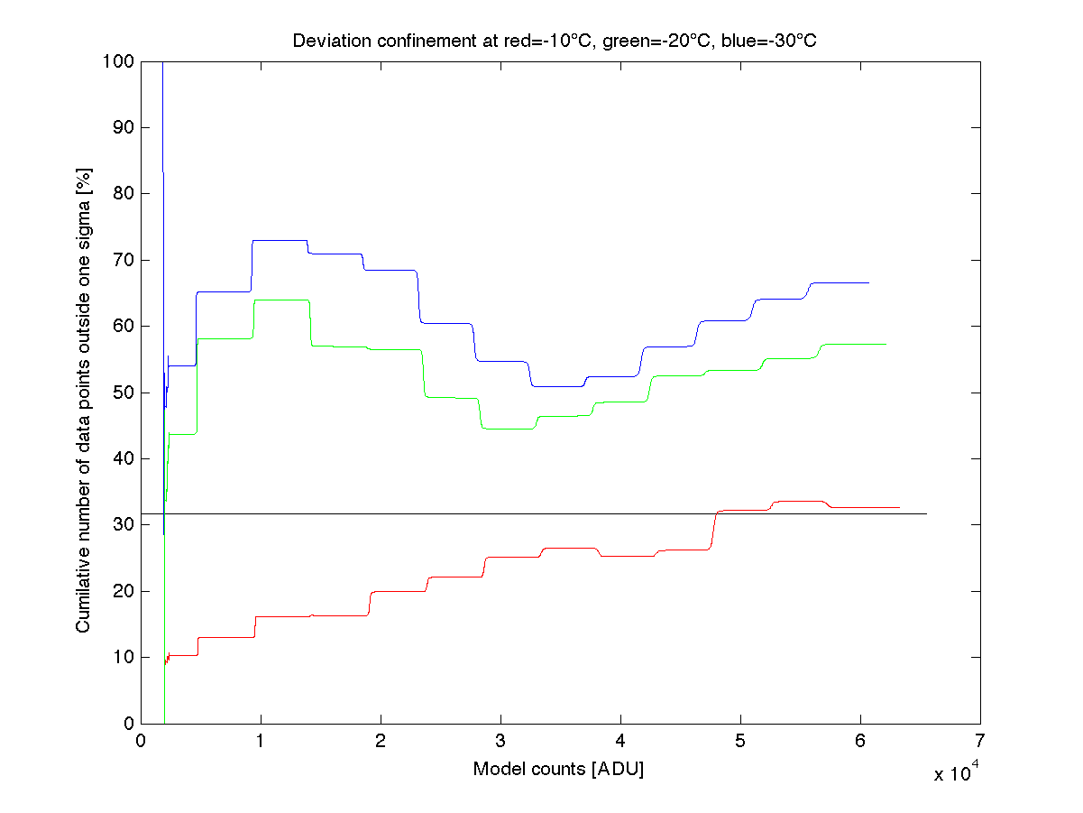
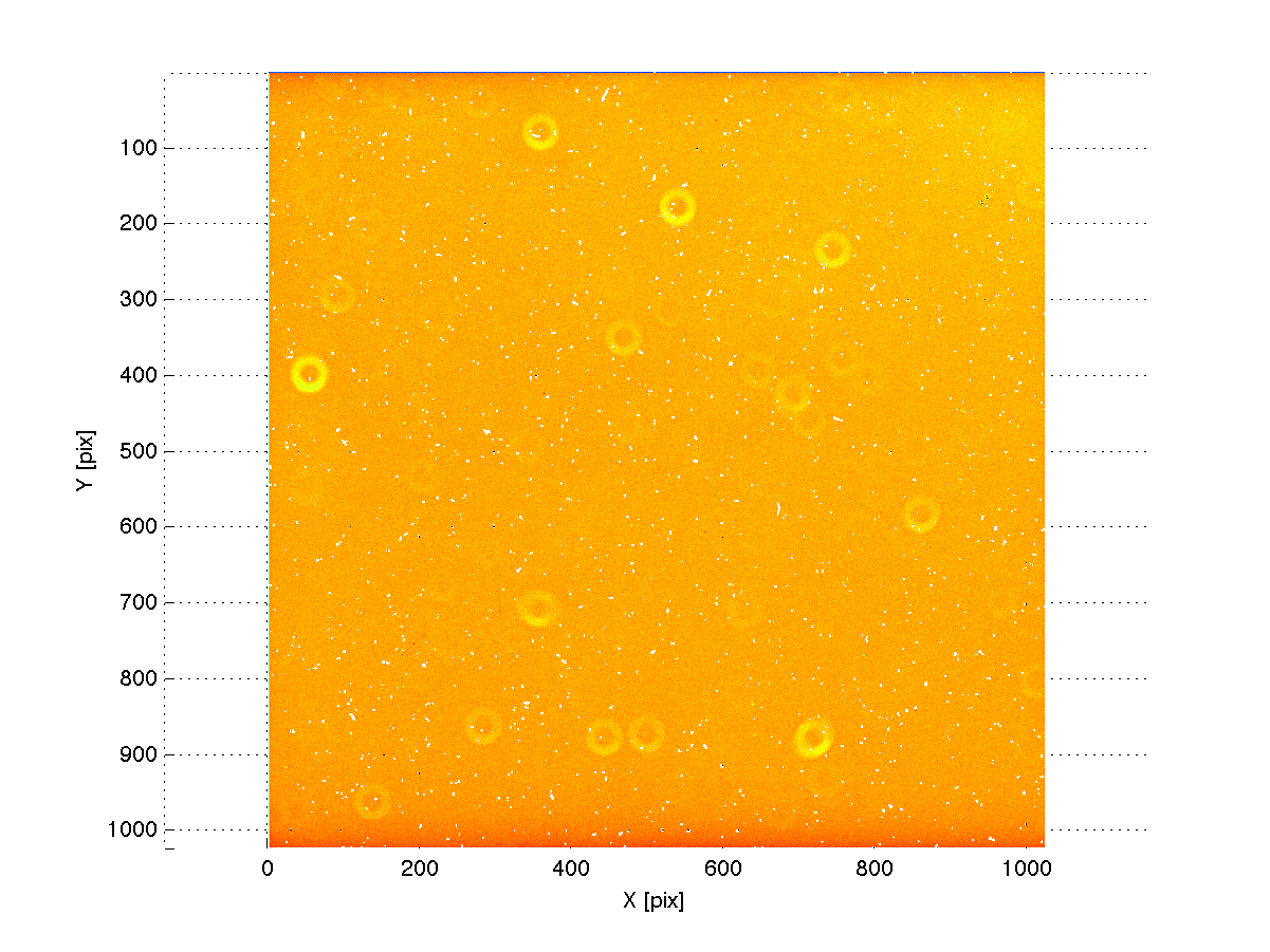
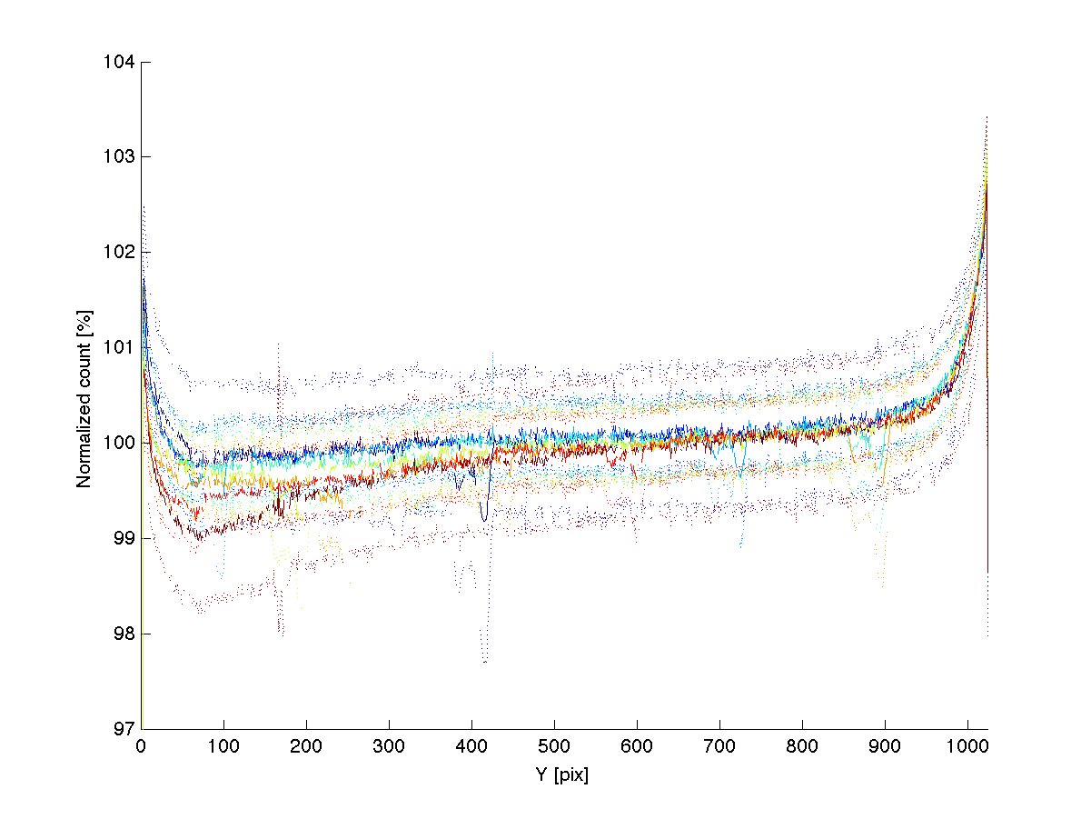
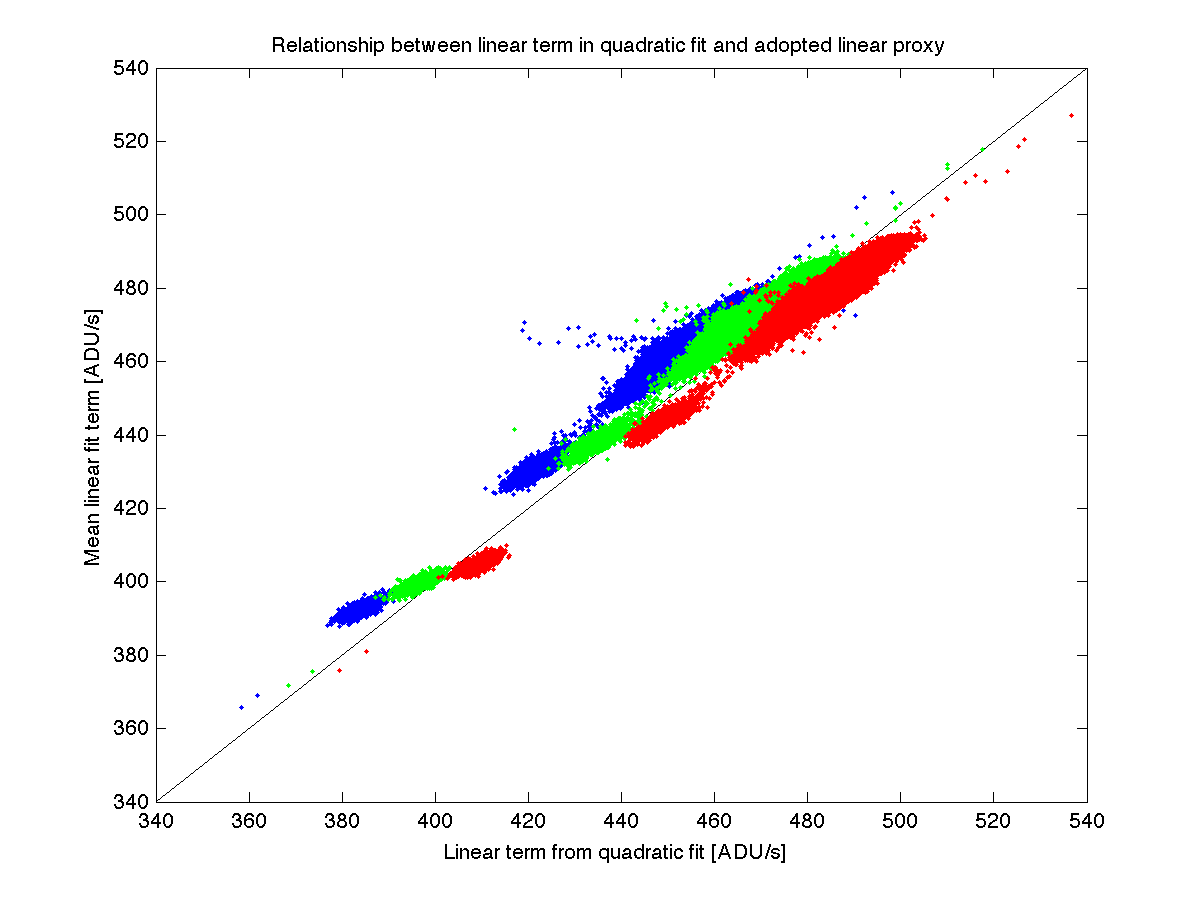
Top left: -10°C case. The data is not particularly well fitted with a linear model. Although most of the data is nomaly within the expected deviation there is a part which is more than one sigma outside. Furthermore, beyond 20,000 counts there are many points which cannot be accounted for by random deviation. Top right: -20°C case. The linear model is a clear compromise between deviation low count data and deviating high count data. Most of the data is not within one sigma deviation from the model. Many data points with more than 10,000 counts are outside the limit for random variations. The largest deviation is larger than for the first set. Bottom left: -30°C case. A majority of the data points have ended up outside of the expected variation for the linear model, especially above 30,000 counts. A lot of points are outside the expected limit for random data variation. This is a direct consequence of the nonlinearity of the data. Bottom right: The cumulative number of points which is outside the one sigma limit (black). The first noisy part is due to low number statistics. All sets have more points outside the one sigma limit than expected. The increasing levels indicates that more points are outside at the higher counts than in the beginning at low counts. The only set which is marginally compatible with random noise is the first set. For the two coolest sets most points are outside the one sigma limit. Some of the noise levels would naturally be reduced in an ordinary reduction process. Here the pixels have not been compensated for their natural variation which would be taken care of by a flat field image. Looking at an image it becomes clear that many of the deviating pixels comes from the edges of the CCD (notice the color of the very edge, blue: low counts, red: high counts, white: masked area). There is also a slight slope (about 0.5%) across the field which can be seen if the image is viewed from the side. This is a consequence of the unevenly light flat field screen. The binned data (128 pixel per bin) along the x-direction (blue to red for increasing x-direction) of the image (solid lines) have uncertainties (dotted lines) of the order 0.5% without any flat field corrections. This is of the same order as the expected shot noise (0.4%) for the mean flux level. Thus, most of the CCD area which would normally be used are likely to have less spread than the given impression from Fig. 6. 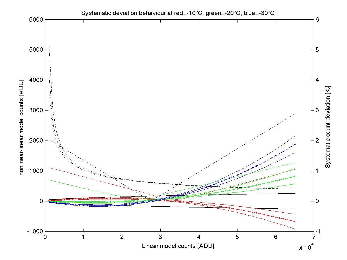 Fig.7 Systematic deviations from linearity. Fig.7 Systematic deviations from linearity.Solid-black: Expected uncertainty from single measurements. Black dashed (-10°C), dash-dotted (-20°C), dotted (-30°C): Uncertainty relative to signal for single measurements(right axis). solid red, green, blue: Quadratic model minus linear model representing systematic deviations from linearity. Dashed red, green, blue: Relative deviation (right axis). It is possible that the second and third of the expected nonlinear effects can be seen in Table 2. For two and four points the uncertainty in the fitted parameters are quite large, but after that there is a decrease in the normalized nonlinear parameter C. This could be an indication that the sensitivity of the CCD first gives a positive parameter A, but that the third effect closer to saturation gradually increases in importance. It should then also be temperature dependent because the decreasing effect is stronger for the warmer cases. The fact that the linear term B increases i.e. the result is a lover value in C, should only have a marginal effect because the change in slope is only around 1%. The relative stability of the slopes B might also point to that a perhaps more true representation of the "true" linear slope. In that case it would be lover than the used value (D). The effect would push the data points to the left and up in Fig 6. making the overall situation worse, as a result of nonlinear effects. In Fig. 7 the result would be that the green and blue solid lines are push up, which in turn would improve the situation at low counts but also lower the limit for the largest number of counts which should be collected in order to approximate a linear relation within uncertainty limits. The limit would then be 30,000 rather than 35,000. 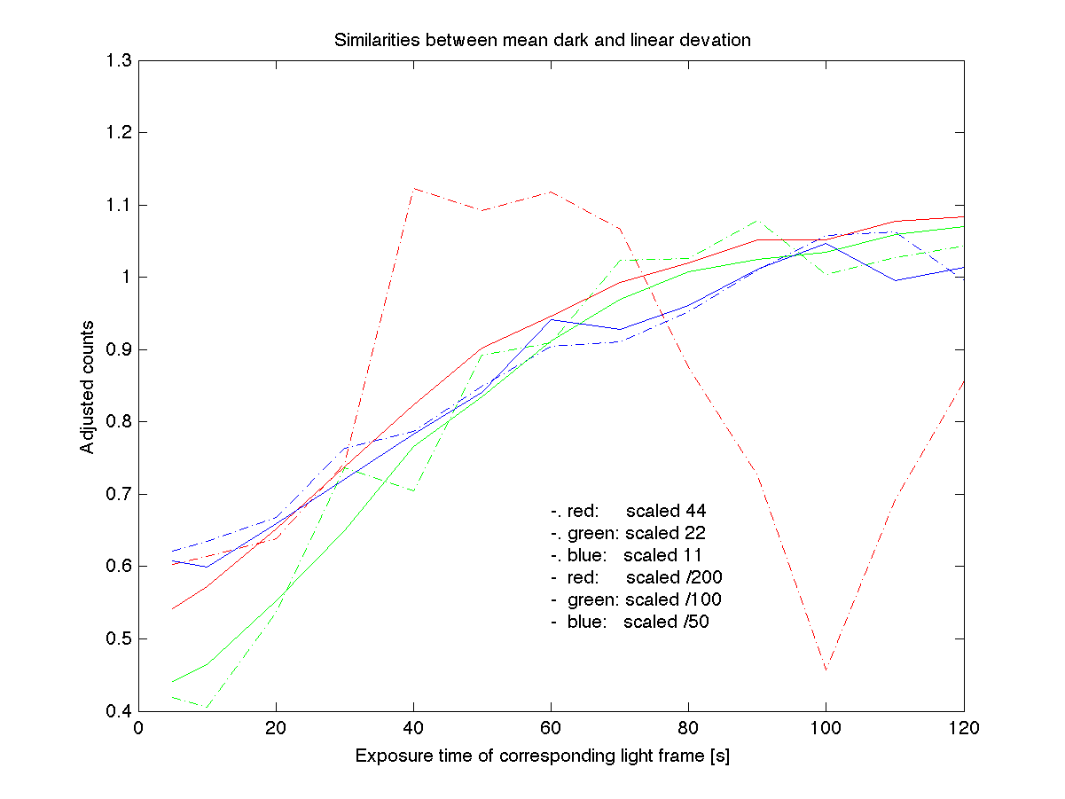 Fig.8 Similarity between DARK count (solid) and nonlinearity in photon count (dash-dotted). The two cooler cases are after a systematic scaling very similar indicating a possible relation while the warmest photon case deviates from the pattern. Fig.8 Similarity between DARK count (solid) and nonlinearity in photon count (dash-dotted). The two cooler cases are after a systematic scaling very similar indicating a possible relation while the warmest photon case deviates from the pattern.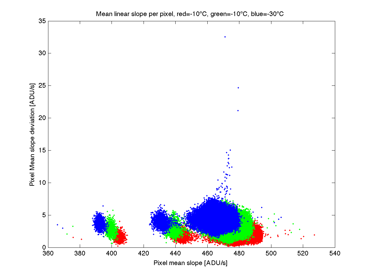 Fig.9 Deviations as a function of slope for the pixel slope proxy (Eq. 7). Each temperature set is shifted in deviation as a result of a stronger nonlinear effect at the lower temperatures. There is also a systematic shift in the slope value which cannot be directly attributed to the nonlinearity. Moreover, the shift is close to linear in appearance. Fig.9 Deviations as a function of slope for the pixel slope proxy (Eq. 7). Each temperature set is shifted in deviation as a result of a stronger nonlinear effect at the lower temperatures. There is also a systematic shift in the slope value which cannot be directly attributed to the nonlinearity. Moreover, the shift is close to linear in appearance.Another plot shows the correlation between the linear terms from Eq. 7 with respect to Eq. 1. |
Discussion |
At this point it is not clear exactly where/why and how the three expected nonlinear effects works. The speculation is that the first case arises by voltage fluctuations possibly related to losses in the power cable and related to the cooling power of the CCD. If it is on the amplifier side (reference voltage) the levels must be stable for more than the readout time of the CCD. Another possibility is that it is a presetting voltage (creating the pixel wells) of the CCD. The cause might also be ripples from the AC/DC conversion. In any case this effect appears to be random-like i.e. compensationable and should be investigated in combination with a battery source and cooling power on/off. The second effect is an increased pixel sensitivity after a previous exposure. It was first thought that this effect arises from saturation, but some testing have shown that even low level exposure leaves a mark. After an exposure the effect is gradually decreasing during a time of at least a couple of hours. Not only is it difficult to test this effect due to the very long relaxing times but in order to compensate for the effect the exposure history during a significant time (perhaps up to hours) must be taken into consideration, if it is even possible to fully map the effect. The third effect is thought to be related to blooming/saturation. Although the camera should not have an anti blooming device the indications are that the pixel sensitivity goes down when closing saturation. The solution to this problem would be to put an upper limit to the number of counts in the pixels which can be regarded as safe from a linearity perspective. The primary aim of this investigation was to find such a limit. Because of the nonlinear behavior it is problematic to use all sky photometry. However, since the first and second nonlinear effect appears to apply to the whole frame and only noticeable between frames, relative photometry should work providing the number of maximum counts in a pixel is held at 30,000 (and no more than 40,000) where the third "near full well" effects might be present. One thing that might cause a problem is if the same area is imaged all the time and stars are held at the same pixels. In that case "bright" stars might gradually become "brighter" due to the second effect. The same should also apply to construction of flatfields where already bright pixels becomes brighter, but if the optical system is already quite flat to begin with then the relative effect should be small. It could perhaps be possible to compensate/cancel the second and third effects with each other around a CCD temperature of -15°C, but this must be checked. |
| Last update : |