Allmost all parameters in the parameter file are valid for the HD and
the MHD module.
Only a few parameters for the hydrodynamics control
(character hdscheme: Sect. 5.4.7,
character reconstruction: Sect. 5.4.7,
real c_slopered: Sect. 5.4.7)
are slightly modified or extended for the MHD module.
character hdscheme:
With this parameter the type of the hydrodynamics scheme can be specified as in
character hdscheme f=A80 b=80 n='Hydrodynamics scheme' &
c0='Roe (approximate Riemann solver of Roe type)' &
c1='RoeMagKin (Roe solver + kinetic magnetic field transport)' &
c2='RoeMHD/HLLMHD (MHD solver)' &
c3='None (skip hydrodynamics step entirely)'
Roe
Possible values are
None: The hydrodynamics step is skipped entirely (for test purposes). Note that in this
case some initializations necessary for the generation of the mean file are omitted, too.
Roe: (default) The standard approximate Riemann solver of Roe-type is activated.
This value will be chosen in most cases.
RoeMagKin: The standard Roe solver is extended to transport passively a magnetic field.
This is a test implementation to check, if the general magnetic field handling
works. For proper MHD simulations use HLLMHD instead.
RoeMHD: Use the MHD Roe solver.
HLLMHD: Use the MHD HLL solver (the current recommend value for MHD simulations).
character hdtimeintegrationscheme:
With this parameter the type of the MHD time-integration scheme can be specified as in
character hdtimeintegrationscheme f=A80 b=80 n='MHD time-integration scheme' &
c0='Hancock' &
c1='Euler1 (default)' &
c2='RungeKutta2'
RungeKutta2
So far, this parameter is only recognized by the HLLMHD scheme.
Possible values are
Hancock: Terms of second order in time are approximated by a Hancock predictor step.
Euler1: (default) A single Euler step is used (only first order in time).
RungeKutta2: A two-step (predictor-corrector) Runge-Kutta step is used.
RungeKutta3: A three-step Runge-Kutta step is used.
character hdsplit:
With this parameter the type of the hydrodynamics
operator (directional) splitting scheme
can be specified as in
character hdsplit f=A80 b=80 n='Hydrodynamics directional splitting scheme' &
c0='123: directional splitting (default)' &
c1='unsplit: new unsplit operator'
123
Possible values are
123: (default) The standard directional splitting is activated,
where the 1D operators for the individual directions are applied in the given order.
So far, only the order 123 is possible.
unsplit: The standard solver is applied.
However, the changes from the individual steps are computed from (and applied to)
the same model configuration. The result is an unsplit scheme.
This parameter is recognized by hdscheme=Roe and hdscheme=HLLMHD.
character hdcheckflux:
With this parameter the CheckFlux routine of the HLLMHD solver can be (des)activated, as e.g. in
character hdcheckflux f=A80 b=80 n='Switch to activate checking of MHD fluxes' &
c0='on/off'
off
This parameter is only recognized by the HLLMHD scheme.
Leaving it on might be safer but is definitely (slightly) slower.
character reconstruction:
This parameter determines the order and ``aggressiveness'' of the reconstruction scheme with e.g.
character reconstruction f=A80 b=80 n='Reconstruction method' &
c0=Constant c1=Minmod/VanLeer/Superbee c2=PP
Minmod
Possible values are
Constant: The run of the partial waves inside the cells is assumed to be constant.
A highly dissipative first order scheme results.
This values will usually only be used for test (or comparison) purposes.
Minmod: Chooses the smallest slope which still results in a second order scheme.
It is the most diffusive (and most stable) one in this class.
VanLeer: (default) The recommended second order scheme.
Superbee: The ``most aggressive'' stable 2nd order scheme.
It results in the steepest shocks, which works well in some test cases
but might be to difficult for the radiation transport module to handle.
PP: Chooses the piecewise parabolic reconstruction of the PPM scheme
(``Piecewise Parabolic Method'', Colella & Woodward 1984).
Results in 3rd order accuracy for the advection.
This method can not be used with hdscheme=HLLMHD.
Usually, the VanLeer reconstruction is a good choice.
If a more stable (and diffusive) scheme is needed, take Minmod.
The PP reconstruction gives the highest accuracy.
However, it tends to produce somewhat ``noisy'' models with small wiggles
e.g. in the velocity.
The 2nd-order piecewise-parabolic reconstruction (PP) is implemented
in the MHD module and gives better results than in the HD module.
By specifying e.g. VanLeer Superbee it is possible to use
the VanLeer scheme for the hydrodynamics scheme as such and Superbee only
for the advection of additional quc quantities.
real c_slopered:
When -Drhd_roe1d_slope_l01=2 is set (see Sect. 3.6),
a new extra stabilization mechanism can be activated:
If one of the reconstruction methods VanLeer, Superbee, or PP
(see Sect. 5.4.7) is activated, the slope can be reduced
(by averaging with the results from a MinMod reconstruction) by setting
c_slopered to a positive non-zero value.
This value can be set e.g. with
real c_slopered f=E15.8 b=4 &
n='Slope reduction parameter in case of strong density contrast' u=1 &
c0='0.00: off (default), 0.02: reasonable value, 0.10: large value'
0.02
Typical choices are
0.0: Slope reduction switched off.
Original reconstruction is used.
0.02: Moderate slope reduction in case of large density jumps.
0.10: More pronounced slope reduction in case of strong density contrast.
This parameter is not recognized by the hdscheme=HLLMHD.
real c_hydpredfactor:
The "hydrostatic pressure correction" terms in the two acoustic waves are
always present.
However, for the entropy wave and the "ionization wave" it is not quite clear
if the terms should be there (the classical default) or if they should be
set to zero.
The value of a factor in front of these terms can be set e.g. with
real c_hydpredfactor f=E15.8 b=4 &
n='hydrostatic pressure reduction in waves 3 and 6' u=1 &
c0='0.0: Deactivation of pressure reduction terms' &
c1='1.0: Activation of pressure reduction terms (default)'
0.0
Possible choices are
0.0: Deactivation of pressure reduction terms
in waves 3 and "6" in Roe solver
1.0: Activation of pressure reduction terms
in waves 3 and "6" in Roe solver (default)
This parameter is not recognized by the MHD module.
integer n_hyditer:
After each complete hydiative time step the recommendation for the next time step
will be chosen so that n_hyditer iterations will (probably) needed.
The parameter can be set e.g. with
integer n_hyditer f=I4 b=4 &
n='Number of hydrodynamics iterations' c0=10
8
For a simulation of a solar-type star it will typically be set to 1.
E.g. for brown dwarfs with shorter hydrodynamical time scales
values around 10 may be considered.
Note, that the hydrodynamics iteration works somewhat differently than
the radiation transport iteration:
in the latter case the size of the actual time step can be determined after
computing the fluxes,
whereas the hydrodynamics step is (possibly) of at least second order in time
and the time step has to be known in advance.
In cas of the MHD module, this can reduce the computation time significantly because
the MHD time step is often much smaller than the other timestep limits.
However, this parameter does not determine the nuber of
substeps directly. Instead, the number of substeps is determined by the
requested timestep and the timestep of each MHD substep which is determined by
the standart Courant condition. So, the number of MHD substeps varies during
the simulation. So, the exact value of this parameter has no direct influence
on the number of substeps. If this parameter is set to zero, this features
is turned of. (See also parameter va_max for speeding up MHD simulations.)
integer n_hydmaxiter:
The absolute maximum number of hydro iterations can be specified e.g. with
integer n_hydmaxiter f=I4 b=4 &
n='Maximum number of hydro iterations' c0=14
0
If more iterations are needed the computation for the current
time step is stopped and resumed with a smaller one.
Usually, n_hydmaxiter will either be set to a value somewhat larger
than the recommended number of iterations (n_hyditer)
or to 0 which disables the check for too many iterations completely.
This can be safely allowed in many cases.
To disable the iteration of the hydrodynamics sub-step set
n_hyditer=0.
In cas of the MHD module, this parameter sets the maximum number of
MHD-substeps. If this parameter is set to zero, the number of MHD substeps
is not limited.
integer n_hydcellsperchunk:
In every directional sub-step neighboring 1D columns are independent from each other.
They can be grouped and computed in chunks of arbitrary size.
The approximate number of grid cells per chunk can be specified e.g. with
integer n_hydcellsperchunk f=I9 b=4 &
n='Number of cells per hydro chunk' &
c0='0 => one 2D slice at a time' &
c1='1 => minimum chunk size (inefficient)' &
c2='2500: reasonable value' &
c3='1000000000: maximum chunk size (inefficient and memory intensive)'
20000
The exact number is determined at run time to get (approximately) equal sizes of the individual
chunks.
The choice of this parameter does not affect the result of the computation but
the memory usage and performance:
Smaller (and more) chunks may result in an optimum cache usage and need the smallest
amount of memory, but result in additional overhead due to frequent subroutine calls.
Bigger (and less) chunks are to be preferred for vector machines and processors
with large caches.
Very rough guide values may be
2500: Pentium III, Core 2 Duo processor
20000: RISC processor
100000: Vector machine
Note: For simulations with activated OpenMP
on a parallel machine the chunk size has to be made small enough to
allow at least as many chunks as processors available. This is
particularly important for models with a small number of grid points
(e.g. 2D models).
An example is given for the Hitachi SR8000 in Sect. 3.7.8.
real c_visdrag:
This viscosity parameter controls the drag force which is (if requested)
applied inside the hydrodynamics routines themselves.
It does not act on velocity gradients as usual viscosity but applies a force proportional to the
velocity itself (but with the opposite sign).
The amount can be specified e.g. with
real c_visdrag f=E15.8 b=4 &
n='Drag viscosity parameter' u=1
0.001
The value gives the fraction the velocity is reduced per time step.
Therefore, reasonable values lie between 0.0 and 1.0.
In almost every case the drag forces will be switched off (c_visdrag=0.0).
If e.g. strong pulsation have to be damped in the initial phase of a simulation
a value around 0.001-0.01 seems appropriate.
real c_visbound:
An additional drag force can be added locally in inflow cells in the outer layer
when the transmitting boundary condition is chosen. The value can be
set e.g. with
real c_visbound f=E15.8 b=4 &
n='Boundary drag viscosity parameter' u=1
0.001
This extra drag force is usually not necessary and should be switched off
(with c_visbound=0.0).
integer n_orderconstrainedtransport:
Order of reconstruction of the electric field in the constrained-transport step.
The parameter can be set e.g. with
integer n_orderconstrainedtransport f=I4 b=4 &
n='Number of hydrodynamics iterations' &
c0='order of reconstruction of electric field in constrained-transport step' &
c1='1: Simple arithmetic average (default), 2: Quadratic interpolation'
2
Possible values:
1: Simple arithmetic average of fluxes (default).
2: Quadratic interpolation of fluxes to the cell edges
This parameter is only recognized by the hdscheme=HLLMHD.
integer n_rescellsperchunk:
The approximate number of grid cells per chunk in the 3D resistivity scheme
can be specified e.g. with
integer n_rescellsperchunk f=I9 b=4 &
n='Number of cells per chunk in resistivity routine' &
c0='0 => one 2D slice at a time' &
c1='1 => minimum chunk size (inefficient)' &
c2='10000: typical value'
20000
The exact number is determined at run time to get (approximately) equal sizes of the individual
chunks.
The choice of this parameter does not affect the result of the computation but
the memory usage and performance:
Smaller (and more) chunks may result in an optimum cache usage and need the smallest
amount of memory, but result in additional overhead due to frequent subroutine calls.
Bigger (and less) chunks are to be preferred for vector machines and processors
with large caches.
real c_rescourant:
The tensor resistivity routines have their own time-step restriction.
The recommended typical time step can be set e.g. with
real c_rescourant f=E15.8 b=4 n='resistivity Courant factor' u=1 &
c0='range: 0.0 < C_resCourant, typically: 0.5'
0.5
real c_rescourantmax:
The absolute upper limit for the resistivity time scale can be set with
real c_rescourantmax f=E15.8 b=4 n='maximum resistivity Courant factor' u=1 &
c0='range: C_resCourant <= C_resCourantmax, typically 1.0'
0.95
Its value should be slightly above c_rescourant.
real c_resB:
This parameter specifies the electric resistivity.
Values between 0.0 and 1.0 may be reasonable.
Higher values are possible but drastically reduce the time step.
The default value is 0.0.
Example:
real c_resb f=E15.8 b=4 &
n='Parameter for numerical resistivity' u=1
0.0
The artificial electric resistivity of [Stone & Pringle (2001)] is used.
It is given by
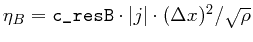 ,
where
,
where  is the magnetic diffusivity,
  the current density,
 a mean width of the grid cell, and
  is the density.
Values
is the density.
Values  disactivate this feature.
real c_resBconst:
This parameter specifies a constant magnetic diffusivity  .
The default value is
.
The default value is 0.0.
Example:
real c_resbconstant f=E15.8 b=4 &
n='Parameter for constant magnetic diffusivity' u=cm^2/s
0.1
A reasonable value can be found by choosing a reasonable value for the magnetic
Reynolds number
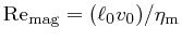 .
Values disactivate this feature.
.
Values disactivate this feature.
real c_resepsilon:
This parameter controls an additional numerical energy diffusion.
Typical values are between 0.0 and 1.0.
The default value is 0.0.
Example:
real c_resepsilon f=E15.8 b=4 &
n='Parameter for additional energy diffusion' u=1
0.5
The diffusion coefficient of the additional energy diffusion is given
by
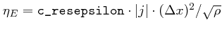 ,
analog to the magnetic diffusivity
,
analog to the magnetic diffusivity c_resB.
Values disactivate this feature.
real beta_inv:
This parameter is used for the dual energy method. It determines
which cells are updated with the thermal energy equation.
Example:
real beta_inv f=E15.8 b=4 &
n='1/beta dual energy parameter' u=1
-1.0
The criterion is as follows:
if
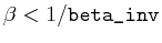 the equation for the thermal energy is used.
if
 the equation for the total energy is used.
 is the plasma , i.e., the ratio of the gas pressure to the
magnetic pressure.
If
is the plasma , i.e., the ratio of the gas pressure to the
magnetic pressure.
If beta_inv is set to zero, the thermal energy equation is used
for all cells. A reasonable value may be 100.0.
To deactivate this feature, set beta_inv to a negative value.
If not specified, this parameter is set to -1.0.
This parameter works only with hdscheme=HLLMHD.
When
 then a reasonable value is given by
 , where
 is the speed of sound in the region where
 .
.
real va_max:
This parameter limits the Alfvén speed to va_max by an arbitrary
reduction of the Lorentz force.
Example:
real va_max f=E15.8 b=4 &
n='maximum Alfven speed' u=cm/s &
-1.0
This parameter is only recognized in conjunction with hdscheme=HLLMHD.
va_max=5.0E+06 might be a reasonable value for some specific
applications to the solar photosphere. If not specified this parameter is
set -1.0. Values disactivate this feature.
See also Eq. 16.
integer N_magDiffSide:
Increases the diffusivity of the scheme near the side boundaries within a
thickness of the diffusion layer of N_magDiffSide computational cells.
Example:
integer n_magdiffside f=I9 b=4 &
n='Number of cells of diffusive side boundary layer' &
c0='0 => deactivates this feature' &
c1='10: reasonable value'
0
integer N_magDiffTop:
Increases the diffusivity of the scheme near the top boundary within a
thickness of the diffusion layer of N_magDiffTop computational cells.
Example:
integer n_magdifftop f=I9 b=4 &
n='Number of cells of diffusive top boundary layer' &
c0='0 => deactivates this feature' &
c1='10: reasonable value'
0
integer N_magDiffBottom:
Increases the diffusivity of the scheme near the bottom boundary within a
thickness of the diffusion layer of N_magDiffBottom computational cells.
Example:
integer n_magdiffbottom f=I9 b=4 &
n='Number of cells of diffusive bottom boundary layer' &
c0='0 => deactivates this feature' &
c1='10: reasonable value'
0