B..1 Linear advection

Exercise:

• Solve the 1D linear advection equation (63) for $v_{} > 0$ and periodic boundary conditions in the interval $[-0.5, 0.5]$ with a set of representative schemes:
  • naive FTCS - Eqs. (92) and (110),
  • donor cell (FTBS) - Eq. (113),
  • Lax-Wendroff - Eq. (116),
  • Fromm - Eq. (118),
  • PLM: Minmod - Eq. (155),
  • PLM: vanLeer - Eq. (156),
  • PLM: Superbee - Eq. (157).
• Test and compare the schemes (see below).
• Write a report containing a few representative plots and a short evaluation of each scheme.

Detailed questions:

• Naive scheme: Check that it is unstable for non-trivial initial conditions if you wait long enough. Nevertheless, could the scheme be used in any way (e.g. for very smooth initial conditions, small time-steps)? Try to find a way by experimenting and/or by examining Eq. (140).
• The stable schemes: Use a Gaussian ( $e^{-\left(x/0.1\right)^2}$) and a rectangle ( $1 \mbox{ for abs}(x) < 0.2 \mbox{ and } 0 \mbox{ elsewhere}$) as initial conditions. Choose a reasonable Courant number and keep it fixed. Simulate a complete revolution ( $\Delta T v = 1$) to facilitate the comparison with the exact final result (= initial condition).
• Compare the results for different resolutions (e.g. 25, 50, 100, 200 grid points).
• Measure the error with the 1-norm

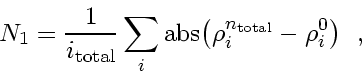  $$N_1 = \frac{1}{i_{\rm total}} \sum_i \mbox{abs} \! \left( \rho_i^{n_{\rm total}} - \rho_i^0 \right) \enspace ,$$ (223)

  the Euclidian 2-norm

  $$N_2 = \frac{1}{i_{\rm total}} \left[ \sum_i \mbox{abs} \! \... ...{n_{\rm total}} - \rho_i^0 \right)^2 \right]^{1/2} \enspace ,$$ (224)

  and the maximum-norm

  $$N_{\max} = \max_i \mbox{abs} \! \left( \rho_i^{n_{\rm total}} - \rho_i^0 \right) \enspace .$$ (225)

• How do the errors decrease with resolution (for the different schemes and initial conditions)?
• How many grid points are needed to preserve a structure (e.g. to push the N2 error below a certain limit)?
• Lax-Wendroff and Fromm scheme: How much overshoot is acceptable? What density contrast in the initial condition can be allowed to be sure that the density remains positive everywhere?
• Perform a numerical FFT analysis (for the lowest resolution and the Gaussian initial condition only). Do the FFT results hint towards instability for the non-linear PLM schemes (particularly Superbee)?