4.4.1 Linearized flux

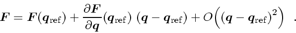
A linearized Riemann solver uses a linearization of the vector flux $\bgroup\color{DEFcolor}$\ensuremath{\mathchoice{\mbox{\boldmath$\displaystyle F$... ...ox{\boldmath$\scriptstyle F$}} {\mbox{\boldmath$\scriptscriptstyle F$}}}$\egroup$ in Eq. (41) around reference value $\bgroup\color{DEFcolor}$\ensuremath{\mathchoice{\mbox{\boldmath$\displaystyle q$... ...\scriptstyle q$}} {\mbox{\boldmath$\scriptscriptstyle q$}}}_\mathrm{ref}$\egroup$ to bring it into a form similar to the scalar Eq. (194),

$\begin{displaymath} \ensuremath{\mathchoice{\mbox{\boldmath$\displaystyle F$}} ... ...ptscriptstyle q$}}}_\mathrm{ref} \right)^2 \right) \enspace . \end{displaymath}$

(203)

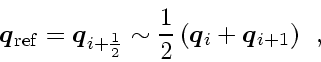
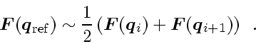
Dropping the 2nd order term and choosing $\bgroup\color{DEFcolor}$x_\mathrm{ref} = x_{i+\frac{1}{2}}$\egroup$ we get

$\begin{displaymath} \ensuremath{\mathchoice{\mbox{\boldmath$\displaystyle q$}} ... ...x{\boldmath$\scriptscriptstyle q$}}}_{i+1} \right) \enspace , \end{displaymath}$

(204)

$\begin{displaymath} \ensuremath{\mathchoice{\mbox{\boldmath$\displaystyle F$}} ... ...ath$\scriptscriptstyle q$}}}_{i+1} \right) \right) \enspace . \end{displaymath}$

(205)

We remember from Sect. 1.5.3 that for the Jacobian

$\begin{displaymath} \bar{\bar{\ensuremath{\mathsf{A}}}}_{i+\frac{1}{2}} := \f... ...{\mbox{\boldmath$\scriptscriptstyle q$}}}_\mathrm{ref} \right) \end{displaymath}$

(206)

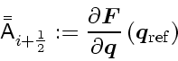
there is a matrix $\bgroup\color{DEFcolor}$\bar{\bar{\ensuremath{\mathsf{Q}}}}_{i+\frac{1}{2}}$\egroup$ that brings it into diagonal form

$\begin{displaymath} \bar{\bar{\ensuremath{\mathsf{\Lambda}}}}_{i+\frac{1}{2}} ... ...bar{\ensuremath{\mathsf{Q}}}}_{i+\frac{1}{2}}^{-1} \enspace . \end{displaymath}$

(207)